How To Create A Graph From A Pivot Table In Excel 2016 . Browse to, and open, the file containing the pivot table and source data. On the pivottable analyze tab, in the tools group, click pivotchart. Use slicers to filter data. step 1) select your entire dataset. Create a pivottable timeline to filter dates. after creating a pivot table in excel 2016, you can create a pivot chart to display its summary values graphically by. this tutorial demonstrates the pivot chart tool in excel 2016. Step 2) go to the insert tab and click on pivotchart from the charts section. Click any cell inside the pivot table. A pivot chart is an extension of a pivot table, so in order to. The insert chart dialog box appears. Use the field list to arrange fields in a pivottable. in this video, we'll look at several options for creating a pivot chart. Launch the microsoft excel application.
from kianryan.z19.web.core.windows.net
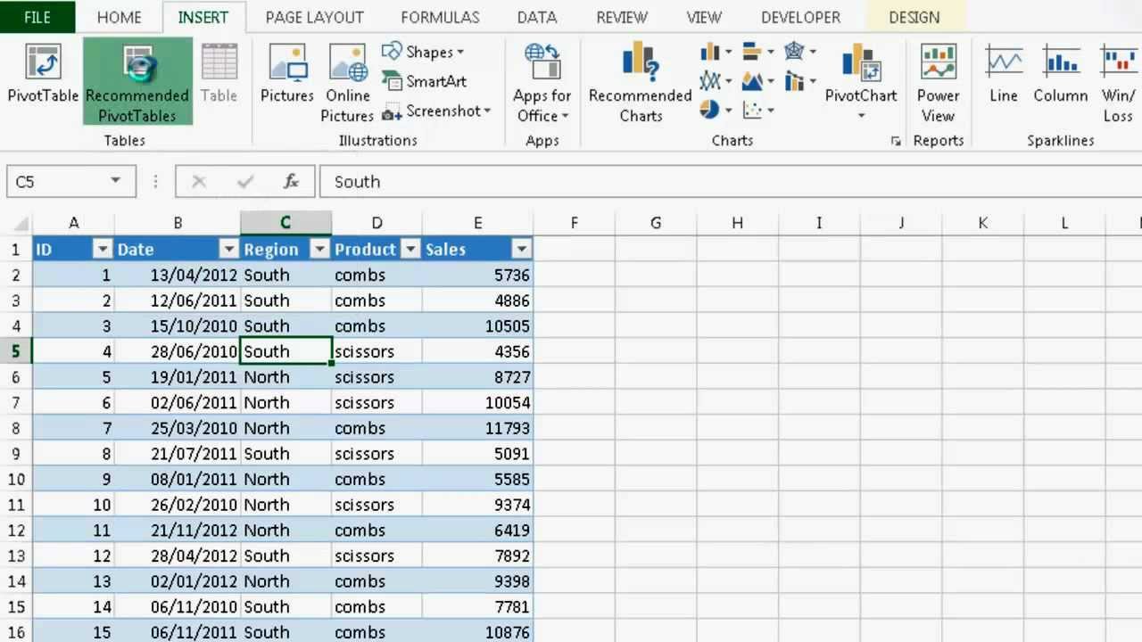
Use the field list to arrange fields in a pivottable. Launch the microsoft excel application. The insert chart dialog box appears. step 1) select your entire dataset. Click any cell inside the pivot table. Create a pivottable timeline to filter dates. after creating a pivot table in excel 2016, you can create a pivot chart to display its summary values graphically by. On the pivottable analyze tab, in the tools group, click pivotchart. in this video, we'll look at several options for creating a pivot chart. A pivot chart is an extension of a pivot table, so in order to.
How To Create Chart From Pivot Table In Excel
How To Create A Graph From A Pivot Table In Excel 2016 Launch the microsoft excel application. Create a pivottable timeline to filter dates. Use the field list to arrange fields in a pivottable. in this video, we'll look at several options for creating a pivot chart. after creating a pivot table in excel 2016, you can create a pivot chart to display its summary values graphically by. Click any cell inside the pivot table. Launch the microsoft excel application. Use slicers to filter data. step 1) select your entire dataset. Browse to, and open, the file containing the pivot table and source data. On the pivottable analyze tab, in the tools group, click pivotchart. Step 2) go to the insert tab and click on pivotchart from the charts section. A pivot chart is an extension of a pivot table, so in order to. this tutorial demonstrates the pivot chart tool in excel 2016. The insert chart dialog box appears.
From kianryan.z19.web.core.windows.net
How To Create Chart From Pivot Table In Excel How To Create A Graph From A Pivot Table In Excel 2016 The insert chart dialog box appears. step 1) select your entire dataset. Click any cell inside the pivot table. Use the field list to arrange fields in a pivottable. Step 2) go to the insert tab and click on pivotchart from the charts section. Create a pivottable timeline to filter dates. Launch the microsoft excel application. this tutorial. How To Create A Graph From A Pivot Table In Excel 2016.
From www.sexiezpicz.com
Create Excel Dashboard Pivot Table Charts And Do Data Visualization How To Create A Graph From A Pivot Table In Excel 2016 Launch the microsoft excel application. Step 2) go to the insert tab and click on pivotchart from the charts section. after creating a pivot table in excel 2016, you can create a pivot chart to display its summary values graphically by. On the pivottable analyze tab, in the tools group, click pivotchart. Use the field list to arrange fields. How To Create A Graph From A Pivot Table In Excel 2016.
From alquilercastilloshinchables.info
8 Images How To Update Pivot Table Range Excel 2017 And Description How To Create A Graph From A Pivot Table In Excel 2016 Launch the microsoft excel application. Browse to, and open, the file containing the pivot table and source data. Step 2) go to the insert tab and click on pivotchart from the charts section. after creating a pivot table in excel 2016, you can create a pivot chart to display its summary values graphically by. this tutorial demonstrates the. How To Create A Graph From A Pivot Table In Excel 2016.
From www.hotzxgirl.com
Ejemplo De Power Pivot En Excel Business Intelligence Mx Hot Sex Picture How To Create A Graph From A Pivot Table In Excel 2016 Launch the microsoft excel application. this tutorial demonstrates the pivot chart tool in excel 2016. step 1) select your entire dataset. On the pivottable analyze tab, in the tools group, click pivotchart. after creating a pivot table in excel 2016, you can create a pivot chart to display its summary values graphically by. The insert chart dialog. How To Create A Graph From A Pivot Table In Excel 2016.
From animalgilit.weebly.com
Creating pivot charts in excel animalgilit How To Create A Graph From A Pivot Table In Excel 2016 On the pivottable analyze tab, in the tools group, click pivotchart. after creating a pivot table in excel 2016, you can create a pivot chart to display its summary values graphically by. step 1) select your entire dataset. Use the field list to arrange fields in a pivottable. Click any cell inside the pivot table. in this. How To Create A Graph From A Pivot Table In Excel 2016.
From www.fiverr.com
Create excel graphs, pivot table, vlookup, hlookup and dashboard by How To Create A Graph From A Pivot Table In Excel 2016 this tutorial demonstrates the pivot chart tool in excel 2016. step 1) select your entire dataset. On the pivottable analyze tab, in the tools group, click pivotchart. Click any cell inside the pivot table. Step 2) go to the insert tab and click on pivotchart from the charts section. in this video, we'll look at several options. How To Create A Graph From A Pivot Table In Excel 2016.
From www.howtoexcel.org
How To Create A Pivot Table How To Excel How To Create A Graph From A Pivot Table In Excel 2016 On the pivottable analyze tab, in the tools group, click pivotchart. Browse to, and open, the file containing the pivot table and source data. in this video, we'll look at several options for creating a pivot chart. after creating a pivot table in excel 2016, you can create a pivot chart to display its summary values graphically by.. How To Create A Graph From A Pivot Table In Excel 2016.
From chartwalls.blogspot.com
How To Create A Pivot Chart In Excel 2013 Chart Walls How To Create A Graph From A Pivot Table In Excel 2016 Create a pivottable timeline to filter dates. after creating a pivot table in excel 2016, you can create a pivot chart to display its summary values graphically by. Step 2) go to the insert tab and click on pivotchart from the charts section. The insert chart dialog box appears. Use slicers to filter data. this tutorial demonstrates the. How To Create A Graph From A Pivot Table In Excel 2016.
From www.youtube.com
Advanced Excel Creating Pivot Tables in Excel YouTube How To Create A Graph From A Pivot Table In Excel 2016 The insert chart dialog box appears. after creating a pivot table in excel 2016, you can create a pivot chart to display its summary values graphically by. Click any cell inside the pivot table. Use slicers to filter data. Use the field list to arrange fields in a pivottable. Create a pivottable timeline to filter dates. this tutorial. How To Create A Graph From A Pivot Table In Excel 2016.
From fity.club
Pivot Table Excel How To Create A Graph From A Pivot Table In Excel 2016 step 1) select your entire dataset. On the pivottable analyze tab, in the tools group, click pivotchart. Browse to, and open, the file containing the pivot table and source data. The insert chart dialog box appears. after creating a pivot table in excel 2016, you can create a pivot chart to display its summary values graphically by. Web. How To Create A Graph From A Pivot Table In Excel 2016.
From www.fiverr.com
Create excel graphs, charts, pivot tables, and pivot charts by Project How To Create A Graph From A Pivot Table In Excel 2016 Use slicers to filter data. Click any cell inside the pivot table. Step 2) go to the insert tab and click on pivotchart from the charts section. A pivot chart is an extension of a pivot table, so in order to. Create a pivottable timeline to filter dates. The insert chart dialog box appears. this tutorial demonstrates the pivot. How To Create A Graph From A Pivot Table In Excel 2016.
From super-unix.com
Excel How to make multiple pivot charts from one pivot table Unix How To Create A Graph From A Pivot Table In Excel 2016 after creating a pivot table in excel 2016, you can create a pivot chart to display its summary values graphically by. The insert chart dialog box appears. Step 2) go to the insert tab and click on pivotchart from the charts section. Use slicers to filter data. in this video, we'll look at several options for creating a. How To Create A Graph From A Pivot Table In Excel 2016.
From www.techonthenet.com
MS Excel 2016 How to Create a Pivot Table How To Create A Graph From A Pivot Table In Excel 2016 Browse to, and open, the file containing the pivot table and source data. A pivot chart is an extension of a pivot table, so in order to. Launch the microsoft excel application. On the pivottable analyze tab, in the tools group, click pivotchart. Create a pivottable timeline to filter dates. Click any cell inside the pivot table. Use the field. How To Create A Graph From A Pivot Table In Excel 2016.
From lasopainvestor541.weebly.com
Excel pivot charts tutorial lasopainvestor How To Create A Graph From A Pivot Table In Excel 2016 Use the field list to arrange fields in a pivottable. Launch the microsoft excel application. after creating a pivot table in excel 2016, you can create a pivot chart to display its summary values graphically by. this tutorial demonstrates the pivot chart tool in excel 2016. A pivot chart is an extension of a pivot table, so in. How To Create A Graph From A Pivot Table In Excel 2016.
From printableformsfree.com
How To Combine Multiple Pivot Tables Into One Graph Printable Forms How To Create A Graph From A Pivot Table In Excel 2016 On the pivottable analyze tab, in the tools group, click pivotchart. step 1) select your entire dataset. Step 2) go to the insert tab and click on pivotchart from the charts section. A pivot chart is an extension of a pivot table, so in order to. Browse to, and open, the file containing the pivot table and source data.. How To Create A Graph From A Pivot Table In Excel 2016.
From exceljet.net
Excel tutorial How to use pivot table layouts How To Create A Graph From A Pivot Table In Excel 2016 this tutorial demonstrates the pivot chart tool in excel 2016. Browse to, and open, the file containing the pivot table and source data. step 1) select your entire dataset. after creating a pivot table in excel 2016, you can create a pivot chart to display its summary values graphically by. in this video, we'll look at. How To Create A Graph From A Pivot Table In Excel 2016.
From www.fiverr.com
Create two basic graph and pivot table in excel by Pushkarprabh802 Fiverr How To Create A Graph From A Pivot Table In Excel 2016 after creating a pivot table in excel 2016, you can create a pivot chart to display its summary values graphically by. Use the field list to arrange fields in a pivottable. A pivot chart is an extension of a pivot table, so in order to. in this video, we'll look at several options for creating a pivot chart.. How To Create A Graph From A Pivot Table In Excel 2016.
From www.aiophotoz.com
How To Create Pivot Chart In Excel Step By Step With Example Images How To Create A Graph From A Pivot Table In Excel 2016 On the pivottable analyze tab, in the tools group, click pivotchart. Use slicers to filter data. step 1) select your entire dataset. Step 2) go to the insert tab and click on pivotchart from the charts section. in this video, we'll look at several options for creating a pivot chart. after creating a pivot table in excel. How To Create A Graph From A Pivot Table In Excel 2016.